Hydra Configuration Management
The following tutorial demonstrates how one may calibrate a simulation model using Hydra configuration files, which calisim incorporates as an optional dependency.
Hydra may be used to specify complex calibration procedures within composable YAML files. We will henceforth provide a basic example.
import numpy as np
import pandas as pd

from calisim.config import HydraConfiguration

import warnings
warnings.filterwarnings("ignore")
YAML Configuration
We will first instantiate a Hydra configuration object. This contains various utility functions for working with Hydra configuration files.
hydra_config = HydraConfiguration()
We will next view the contents of the conf directory, which contains the config.yaml file, alongside three subdirectories:
calibration
metric
model
! ls conf
calibration config.yaml metric model
The contents of config.yaml are as follows:
defaults:
  - _self_
  - calibration: lotka_optimisation
  - model: lotka_volterra
  - metric: mse
We can see that the three elements within the defaults list (calibration, model, metric) match the three subdirectory names above. Let’s look at the files within the metric subdirectory.
! ls conf/metric
mse.yaml
We see a YAML file called mse.yaml, which matches the value of the metric element in the defaults list.
defaults:
  ...
  - metric: mse
The contents of the mse.yaml are as follows:
_target_: calisim.statistics.MeanSquaredError
Similarly, the model subdirectory contains a YAML file called lotka_volterra.yaml which is composed of the following:
_target_: calisim.example_models.LotkaVolterraModel
This should give you an idea of how Hydra works. Hydra will instantiate a configuration dictionary containing three keys (calibration, model, metric) The metric key will be mapped to a MeanSquaredError object while the model key will be mapped to a LotkaVolterraModel object.
But how about the the calibration key? Referring to the defaults list again:
defaults:
  - _self_
  - calibration: lotka_optimisation
Within the calibration subdirectory, there exists a YAML file called lotka_optimisation.yaml. This file a bit more complicated:
_target_: calisim.optimisation.OptimisationMethod
_partial_: true
engine: emukit
specification:
    _target_: calisim.optimisation.OptimisationMethodModel
    experiment_name: emukit_optimisation
    parameter_spec:
        parameters:
            - name: alpha
              distribution_name: uniform
              distribution_args: [0.45, 0.55]
              data_type: continuous
            - name: beta
              distribution_name: uniform
              distribution_args: [0.02, 0.03]
              data_type: continuous
    directions: [ minimize ]
    output_labels: [ Lynx ]
    acquisition_func: ei
    n_iterations: 25
    n_init: 20
    n_samples: 100
    n_out: 1
    verbose: false
    method_kwargs:
        noise_var: 0.001
So, the calibration key is mapped to an OptimisationMethod object that uses the emukit engine. Under specification, we can see the parameter_spec containing parameter distribution information, the acquisition function (ei), the number of iterations (25), and so on. However, the OptimisationMethod object has a mandatory argument within its constructor called calibration_func, which we have not defined in the YAML file (note that it is possible to specify a particular calibration function by providing its full module path and name). In order to instantiate OptimisationMethod, we include _partial_: true so that we can dynamically specify calibration_func within our Python code.
Instantiation
Let’s construct a raw configuration object from the config.yaml file.
cfg = hydra_config.get_raw_config("config", "conf")
print(hydra_config.pretty(cfg))
calibration:
  _target_: calisim.optimisation.OptimisationMethod
  _partial_: true
  engine: emukit
  specification:
    _target_: calisim.optimisation.OptimisationMethodModel
    experiment_name: emukit_optimisation
    parameter_spec:
      parameters:
      - name: alpha
        distribution_name: uniform
        distribution_args:
        - 0.45
        - 0.55
        data_type: continuous
      - name: beta
        distribution_name: uniform
        distribution_args:
        - 0.02
        - 0.03
        data_type: continuous
    directions:
    - minimize
    output_labels:
    - Lynx
    acquisition_func: ei
    n_iterations: 25
    n_init: 20
    n_samples: 100
    n_out: 1
    verbose: false
    method_kwargs:
      noise_var: 0.001
model:
  _target_: calisim.example_models.LotkaVolterraModel
metric:
  _target_: calisim.statistics.MeanSquaredError
This contains the contents of the aforementioned YAML files within a single dictionary. However, we can instead construct a configuration object and instantiate all of the classes mapped to the _target_ keys.
cfg = hydra_config.get_configuration("config", "conf")
metric = cfg["metric"]
type(metric)
calisim.statistics.discrepancy.MeanSquaredError
model = cfg["model"]
observed_data = model.get_observed_data()
type(model)
calisim.example_models.lotka_volterra.LotkaVolterraModel
You can see that we have instantiated MeanSquaredError and LotkaVolterraModel objects. Note that we can also override the contents of the YAML configuration files.
For instance, we can instead instantiate a RootMeanSquaredError metric object like so:
cfg = hydra_config.get_configuration(
    "config", "conf",
    overrides=["metric._target_=calisim.statistics.RootMeanSquaredError"]
)
metric = cfg["metric"]
type(metric)
calisim.statistics.discrepancy.RootMeanSquaredError
Hydra enables us to compose highly complex calibration workflows by mixing, matching, and overriding various sets of YAML files and keys. It is certainly possible to implement much more complicated configuration specifications, though we will keep things simple for this tutorial.
Calibration
Let’s next define our objective function for calibration.
def objective(
	parameters: dict, simulation_id: str, observed_data: np.ndarray | None, t: pd.Series
) -> float | list[float]:
	simulation_parameters = dict(h0=34.0, l0=5.9, t=t, gamma=0.84, delta=0.026)

	for k in ["alpha", "beta"]:
		simulation_parameters[k] = parameters[k]

	simulated_data = model.simulate(simulation_parameters).lynx.values
	discrepancy = metric.calculate(observed_data, simulated_data)
	return discrepancy
Finally, we can instantiate a calibrator object, then specify, execute, and analyzea calibration workflow. As mentioned prior, we must dynamically specify the calibration_func in the calibrator’s constructor using our objective function.
calibrator = cfg["calibration"](calibration_func=objective)
calibrator.specification.calibration_func_kwargs=dict(t=observed_data.year)
calibrator.specification.observed_data=observed_data.lynx.values
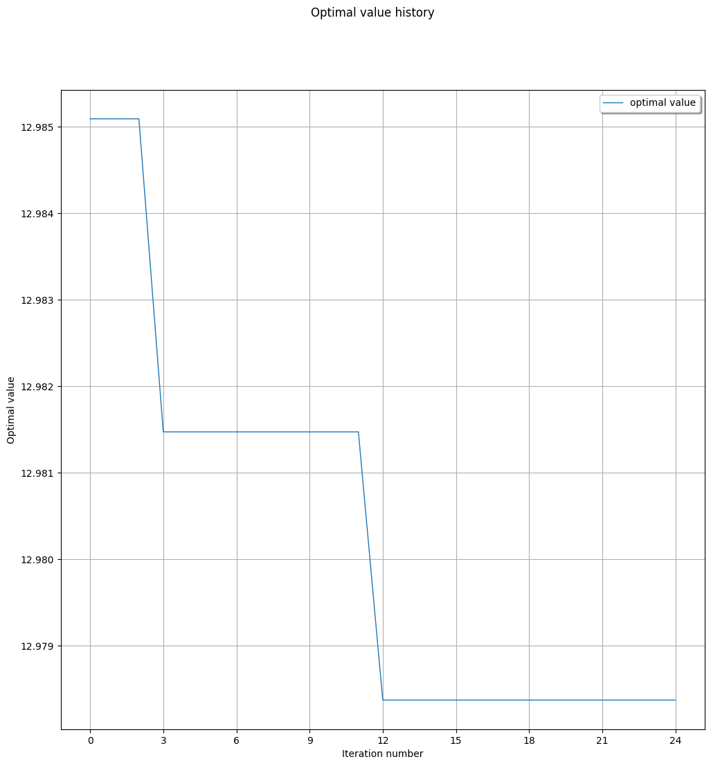
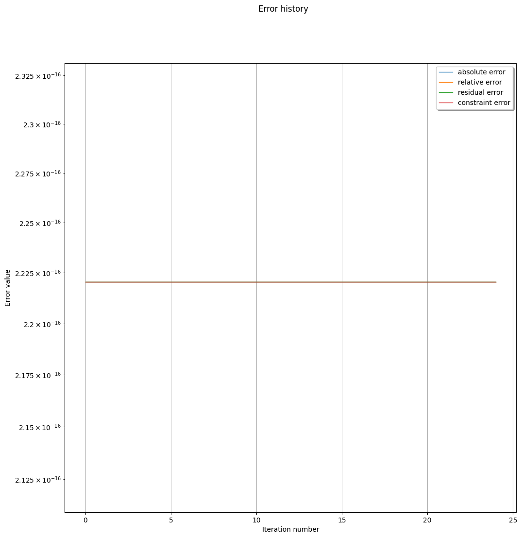
calibrator.specify().execute().analyze()
<calisim.optimisation.implementation.OptimisationMethod at 0x7f6a64149b40>
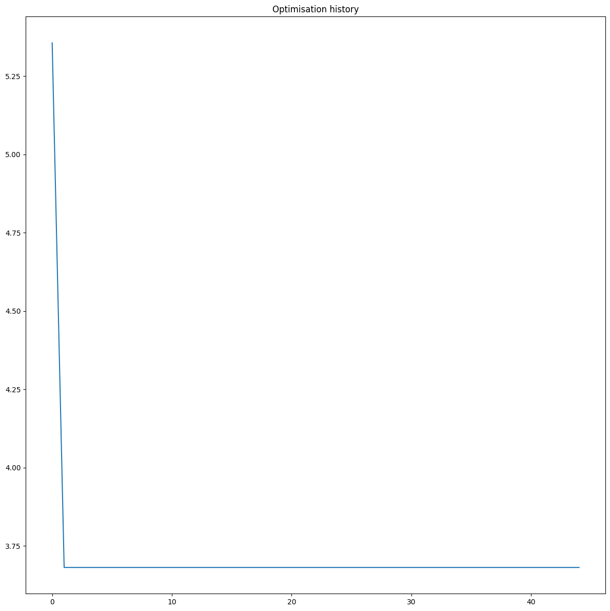
The optimiser is able to retrieve the ground-truth parameter values from our simulation study.
pd.DataFrame([
    { "parameter": estimate.name, "estimate": estimate.estimate, "ground truth": model.GROUND_TRUTH[estimate.name] }
    for estimate in calibrator.get_parameter_estimates().estimates
])
| parameter | estimate | ground truth | |
|---|---|---|---|
| 0 | alpha | 0.518041 | 0.520 |
| 1 | beta | 0.024410 | 0.024 |
Let’s repeat the calibration procedure. But this time, we shall use a Kriging surrogate model for Bayesian optimisation via the openturns engine. Pulling all the above code together:
cfg = hydra_config.get_configuration(
    "config",
    "conf",
    overrides=[
        "calibration.engine=openturns",
        "+calibration.specification.method=kriging",
        "calibration.specification.method_kwargs=null"
    ]
)
metric = cfg["metric"]
model = cfg["model"]
observed_data = model.get_observed_data()

def objective(
	parameters: dict, simulation_id: str, observed_data: np.ndarray | None, t: pd.Series
) -> float | list[float]:
	simulation_parameters = dict(h0=34.0, l0=5.9, t=t, gamma=0.84, delta=0.026)

	for k in ["alpha", "beta"]:
		simulation_parameters[k] = parameters[k]

	simulated_data = model.simulate(simulation_parameters).lynx.values
	discrepancy = metric.calculate(observed_data, simulated_data)
	return discrepancy

calibrator = cfg["calibration"](calibration_func=objective)
calibrator.specification.calibration_func_kwargs=dict(t=observed_data.year)
calibrator.specification.observed_data=observed_data.lynx.values
calibrator.specify().execute().analyze()
<calisim.optimisation.implementation.OptimisationMethod at 0x7f6a6414bdf0>
pd.DataFrame([
    { "parameter": estimate.name, "estimate": estimate.estimate, "ground truth": model.GROUND_TRUTH[estimate.name] }
    for estimate in calibrator.get_parameter_estimates().estimates
])
| parameter | estimate | ground truth | |
|---|---|---|---|
| 0 | alpha | 0.511805 | 0.520 |
| 1 | beta | 0.024113 | 0.024 |
We can see that OpenTurns is also able to recover the ground truth parameters.