TorchX Job Launcher

The following tutorial demonstrates how one may dispatch simulations using the TorchX job launcher, which calisim incorporates as an optional dependency.

TorchX may be used to specify and launch simulations in a distributed and parallelised fashion across different computational environments and backends (AWS, Ray, SLURM, Kubernetes). We will henceforth provide a basic example.

import numpy as np
import pandas as pd
import os
import os.path as osp
import torchx

from calisim.data_model import OrchestrationModel
from calisim.orchestration import TorchXJobLauncher
from calisim.data_model import (
	DistributionModel,
	ParameterDataType,
	ParameterSpecification,
)
from calisim.abc import (
	ApproximateBayesianComputationMethod,
	ApproximateBayesianComputationMethodModel,
)
from calisim.statistics import L2Norm

import warnings
warnings.filterwarnings("ignore")

Dispatching Python-Based Simulations

We will first define a Python command to be called externally by TorchX. We will later demonstrate that calisim is agnostic to your choice of programming language, and can be used to calibration non-Python based models - assuming that they can be called externally and supplied with parameters.

This Python command will execute the Rastrigin function, which will act as our simulation model.

cmd = """
import sys
import numpy as np
import os.path as osp

def rastrigin(x, A=10):
    x = np.array(x)
    n = len(x)
    return A * n + np.sum(x**2 - A * np.cos(2 * np.pi * x))

file_name = sys.argv[1]
x1 = float(sys.argv[2])
x2 = float(sys.argv[3])
x3 = float(sys.argv[4])

x = [x1, x2, x3]

fx = rastrigin(x)
with open(osp.join('data', file_name), 'w') as f:
    f.write(str(fx))    
"""

Our implementation of Rastrigin will make use of three parameters, which are supplied as command line arguments. We next define an OrchestrationModel data model, which contains the parameters needed to launch the TorchX job.

orchestration = OrchestrationModel(
    name="rastrigin",
    entrypoint="python",
    cpu=1,
    memMB=50,
    scheduler="local_cwd",
    time="00:01:59",
    wait_interval=10
)

Referring to the arguments supplied to the OrchestrationModel constructor, we must supply a command entrypoint, which is python in our case such that we can execute a Python command. We require 1 CPU, request 50MB of memory, dispatch the job as a local command using the local_cwd job scheduler, leave up to 2 minutes (00:01:59) to complete the job, and check on the progress of the job every 10 seconds.

We next define the ground truth parameters for a simulation study.

ground_truth=dict(
    x1=0.5,
    x2=1.0,
    x3=-0.7
)

pd.DataFrame(ground_truth, index=[0])

	x1	x2	x3
0	0.5	1.0	-0.7

We’ll make use of the TorchXJobLauncher utility class to launch a Python job with our ground truth parameteters. We’ll supply an instance of the OrchestrationModel class, alongside command line arguments to the job launcher. These arguments must be supplied as a list.

runner = TorchXJobLauncher()
file_name = "ground_truth"
simulation_parameters = list(ground_truth.values())

job_results = runner.launch(
    orchestration, 
    ["-c", cmd, file_name] + simulation_parameters
)
job_results["state"]

SUCCEEDED (4)

The job appears to have succeeded. We can load and view the contents of the simulation output file like so:

file_path = osp.join('data', file_name)
with open(file_path, 'r') as f:
    fx = f.read()  
if os.path.exists(file_path):
    os.remove(file_path)
observed_data = np.array([float(fx)])
observed_data

array([34.83016994])

We will define a ParameterSpecification for the three parameters of the Rastrigin function.

parameter_spec = ParameterSpecification(
	parameters=[
		DistributionModel(
			name="x1",
			distribution_name="normal",
			distribution_args=[0.5, 0.05],
			data_type=ParameterDataType.CONTINUOUS,
		),
		DistributionModel(
			name="x2",
			distribution_name="normal",
			distribution_args=[1.0, 0.05],
			data_type=ParameterDataType.CONTINUOUS,
		),
		DistributionModel(
			name="x3",
			distribution_name="normal",
			distribution_args=[-0.7, 0.05],
			data_type=ParameterDataType.CONTINUOUS,
		),
	]
)

We will next define a calibration function for Appproximate Bayesian Computation.

def abc_func(
	parameters: dict, simulation_id: str, observed_data: np.ndarray | None
) -> float | list[float]:
    simulation_parameters = list(parameters.values())
    file_name = simulation_id
    runner.launch(
        orchestration, 
        ["-c", cmd, file_name] + simulation_parameters
    )
    
    file_path = osp.join('data', file_name)
    with open(file_path, 'r') as f:
        fx = f.read()  
    if os.path.exists(file_path):
        os.remove(file_path)
    
    simulated_data = np.array([float(fx)])
    metric = L2Norm()
    discrepancy = metric.calculate(observed_data, simulated_data)
    return discrepancy

Finally, we will perform Bayesian calibration for the Rastrigin function, demonstrating that calisim can incorporate TorchX to dispatch simulations as jobs.

specification = ApproximateBayesianComputationMethodModel(
	experiment_name="pyabc_approximate_bayesian_computation",
	parameter_spec=parameter_spec,
	observed_data=observed_data,
	n_init=25,
	walltime=1,  
	epsilon=0.1,
	output_labels=["rastrigin"],
	n_bootstrap=15,
    n_jobs=10,
	min_population_size=5,
	verbose=True,
	batched=False,
	method_kwargs=dict(
		max_total_nr_simulations=100, max_nr_populations=20, min_acceptance_rate=0.0
	),
)

calibrator = ApproximateBayesianComputationMethod(
	calibration_func=abc_func, specification=specification, engine="pyabc"
)

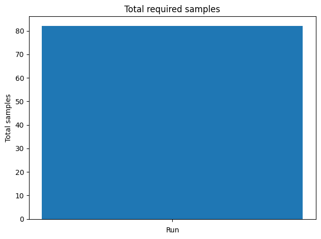
calibrator.specify().execute().analyze()

ABC.Sampler INFO: Parallelize sampling on 10 processes.
ABC.History INFO: Start <ABCSMC id=1, start_time=2026-04-12 16:05:13>
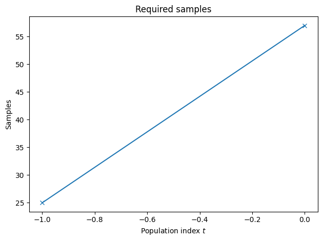
ABC INFO: Calibration sample t = -1.
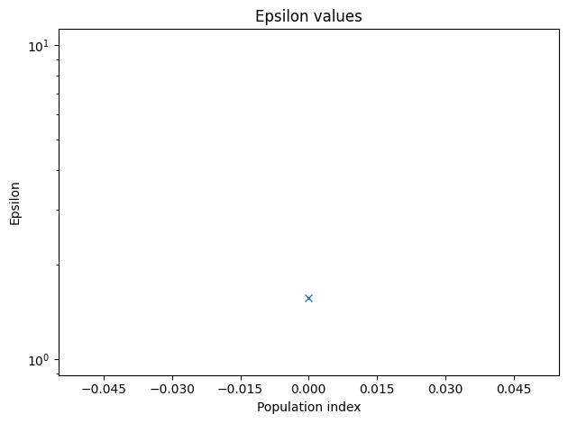
ABC INFO: t: 0, eps: 1.56318334e+00.
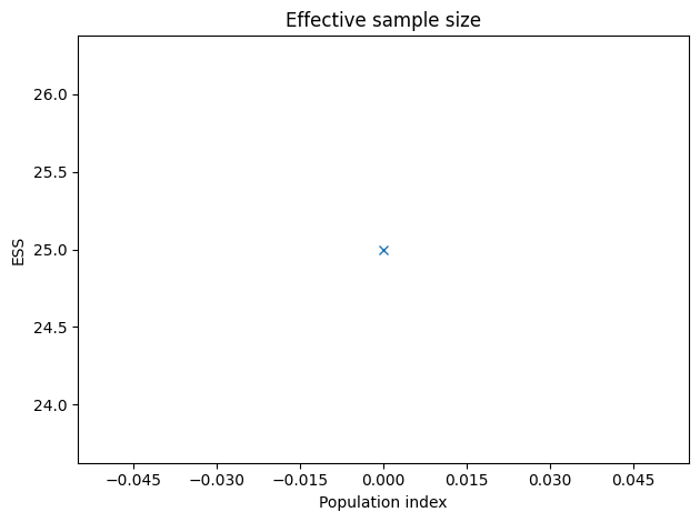
ABC INFO: Accepted: 25 / 57 = 4.3860e-01, ESS: 2.5000e+01.
ABC.Adaptation INFO: Change nr particles 25 -> 10
ABC INFO: Stop: Maximum walltime.
ABC.History INFO: Done <ABCSMC id=1, duration=0:01:44.958505, end_time=2026-04-12 16:06:58>

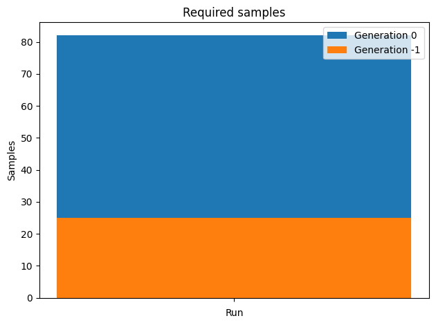
<calisim.abc.implementation.ApproximateBayesianComputationMethod at 0x7fc2218811b0>

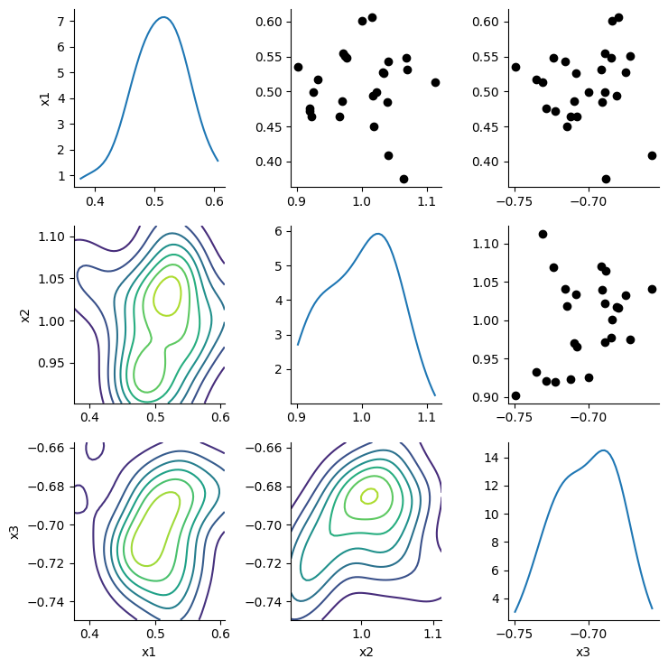
The calibrator is able to retrieve the ground-truth parameter values from our simulation study.

pd.DataFrame([
    { "parameter": estimate.name, "estimate": estimate.estimate, "ground truth": ground_truth[estimate.name] }
    for estimate in calibrator.get_parameter_estimates().estimates
])

	parameter	estimate	ground truth
0	x1	0.507080	0.5
1	x2	0.998336	1.0
2	x3	-0.701737	-0.7

Overall, TorchX is not required for computationally light-weight functions such as our three parameter, Python-based, Rastrigin function. However, it is more useful for running non-Python simulation models which will need to be called externally, along with computationally demanding simulations that must be executed in a distributed and parallelised fashion within a computing cluster.

Dispatching R-Based Simulations

We will next define an R script to be called externally by TorchX, thereby demonstrating that calisim is agnostic to your choice of programming language.

This R script will execute the Rastrigin function, which will act as our simulation model.

cmd = """
rastrigin <- function(x, A=10) {
  n <- length(x)
  A*n + sum(x^2 - A*cos(2*pi*x))
}

args <- commandArgs(trailingOnly=TRUE)
file_name <- args[1]
x <- as.numeric(args[2:4])

out_path <- file.path("data", file_name)
fx <- rastrigin(x)
write(fx, file=out_path)
"""

r_script = "rastrigin.R"
if not os.path.exists(r_script):
    with open(r_script, 'w') as f:
        f.write(cmd)    

Our implementation of Rastrigin will make use of three parameters, which are supplied as command line arguments. We next define an OrchestrationModel data model, which contains the parameters needed to launch the TorchX job.

orchestration = OrchestrationModel(
    name="rastrigin",
    entrypoint="Rscript",
    cpu=1,
    memMB=50,
    scheduler="local_cwd",
    time="00:01:59",
    wait_interval=10
)

You can see that this is nearly identical to the OrchestrationModel for the Python-based implementation of Rastrigin. However, note that we have changed the job entrypoint to Rscript as we are no longer using Python. We will run the code above using the Rscript command to execute an R script.

We next define the ground truth parameters for a simulation study.

ground_truth=dict(
    x1=0.5,
    x2=1.0,
    x3=-0.7
)

pd.DataFrame(ground_truth, index=[0])

	x1	x2	x3
0	0.5	1.0	-0.7

We’ll make use of the TorchXJobLauncher utility class to launch an R job with our ground truth parameteters. We’ll supply an instance of the OrchestrationModel class, alongside command line arguments to the job launcher. These arguments must be supplied as a list.

runner = TorchXJobLauncher()
file_name = "ground_truth"
simulation_parameters = list(ground_truth.values())

job_results = runner.launch(
    orchestration, 
    [r_script, file_name] + simulation_parameters
)
job_results["state"]

SUCCEEDED (4)

The job appears to have succeeded. We can load and view the contents of the simulation output file like so:

file_path = osp.join('data', file_name)
with open(file_path, 'r') as f:
    fx = f.read()  
if os.path.exists(file_path):
    os.remove(file_path)
observed_data = np.array([float(fx)])
observed_data

array([34.83017])

We will define a ParameterSpecification for the three parameters of the Rastrigin function.

parameter_spec = ParameterSpecification(
	parameters=[
		DistributionModel(
			name="x1",
			distribution_name="normal",
			distribution_args=[0.5, 0.05],
			data_type=ParameterDataType.CONTINUOUS,
		),
		DistributionModel(
			name="x2",
			distribution_name="normal",
			distribution_args=[1.0, 0.05],
			data_type=ParameterDataType.CONTINUOUS,
		),
		DistributionModel(
			name="x3",
			distribution_name="normal",
			distribution_args=[-0.7, 0.05],
			data_type=ParameterDataType.CONTINUOUS,
		),
	]
)

We will next define a calibration function for Appproximate Bayesian Computation.

def abc_func(
	parameters: dict, simulation_id: str, observed_data: np.ndarray | None
) -> float | list[float]:
    simulation_parameters = list(parameters.values())
    file_name = simulation_id
    job_results = runner.launch(
        orchestration, 
        [r_script, file_name] + simulation_parameters
    )
    
    file_path = osp.join('data', file_name)
    with open(file_path, 'r') as f:
        fx = f.read()  
    if os.path.exists(file_path):
        os.remove(file_path)
    
    simulated_data = np.array([float(fx)])
    metric = L2Norm()
    discrepancy = metric.calculate(observed_data, simulated_data)
    return discrepancy

Finally, we will perform Bayesian calibration for the Rastrigin function, demonstrating that calisim can incorporate TorchX to dispatch simulations as jobs.

specification = ApproximateBayesianComputationMethodModel(
	experiment_name="pyabc_approximate_bayesian_computation",
	parameter_spec=parameter_spec,
	observed_data=observed_data,
	n_init=25,
	walltime=1,  
	epsilon=0.1,
	output_labels=["rastrigin"],
	n_bootstrap=15,
    n_jobs=10,
	min_population_size=5,
	verbose=True,
	batched=False,
	method_kwargs=dict(
		max_total_nr_simulations=100, max_nr_populations=20, min_acceptance_rate=0.0
	),
)

calibrator = ApproximateBayesianComputationMethod(
	calibration_func=abc_func, specification=specification, engine="pyabc"
)

calibrator.specify().execute().analyze()

ABC.Sampler INFO: Parallelize sampling on 10 processes.
ABC.History INFO: Start <ABCSMC id=1, start_time=2026-04-12 16:07:12>
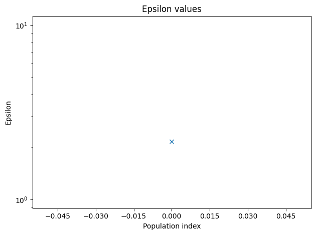
ABC INFO: Calibration sample t = -1.
ABC INFO: t: 0, eps: 2.15310000e+00.
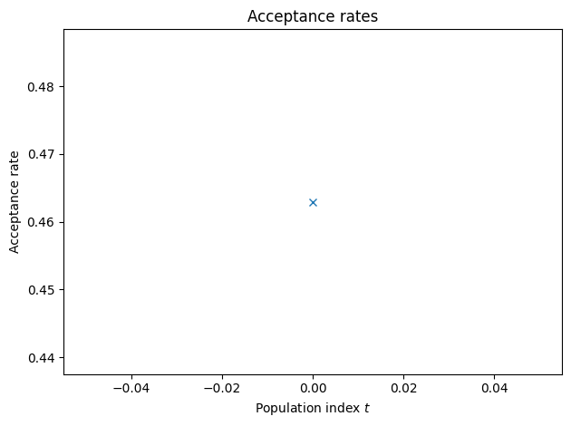
ABC INFO: Accepted: 25 / 54 = 4.6296e-01, ESS: 2.5000e+01.
ABC.Adaptation INFO: Change nr particles 25 -> 10
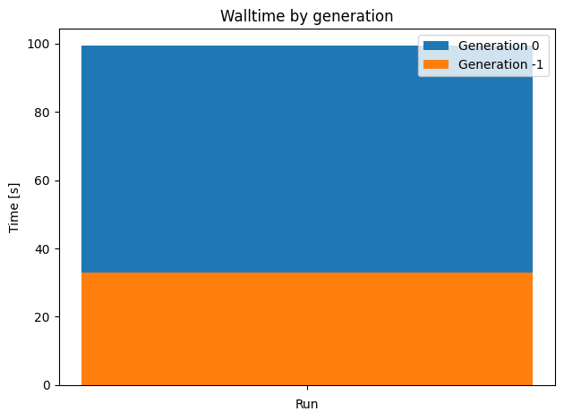
ABC INFO: Stop: Maximum walltime.
ABC.History INFO: Done <ABCSMC id=1, duration=0:01:43.556549, end_time=2026-04-12 16:08:56>

<calisim.abc.implementation.ApproximateBayesianComputationMethod at 0x7fc3546e5390>

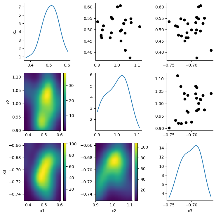
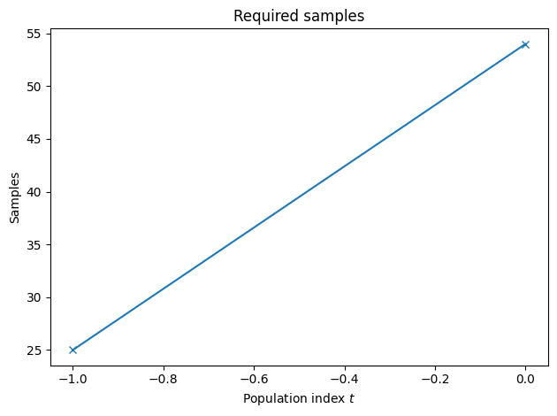
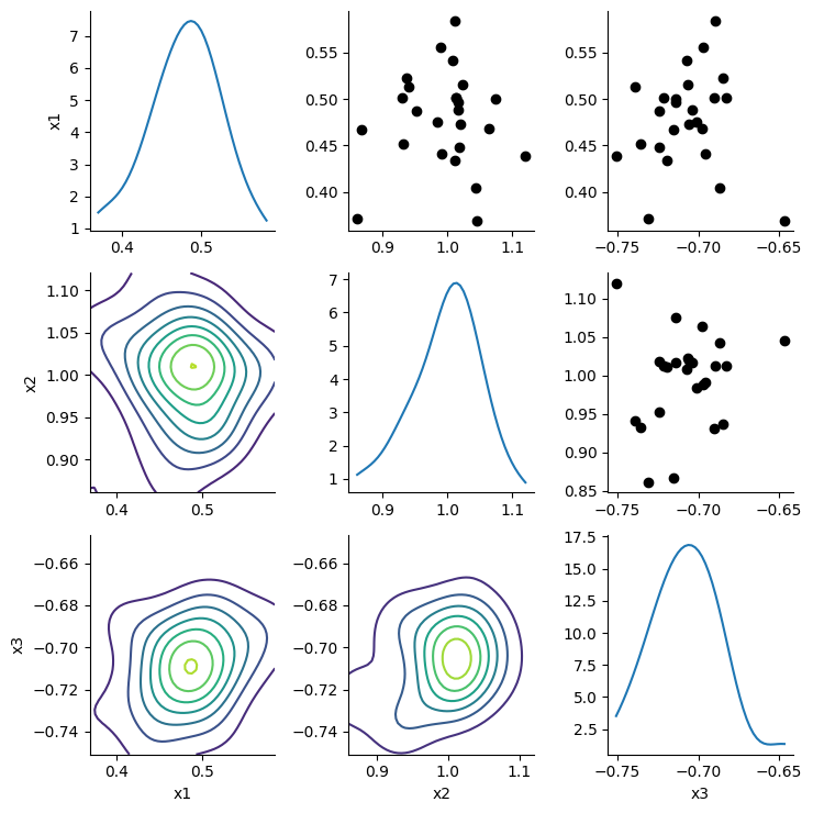
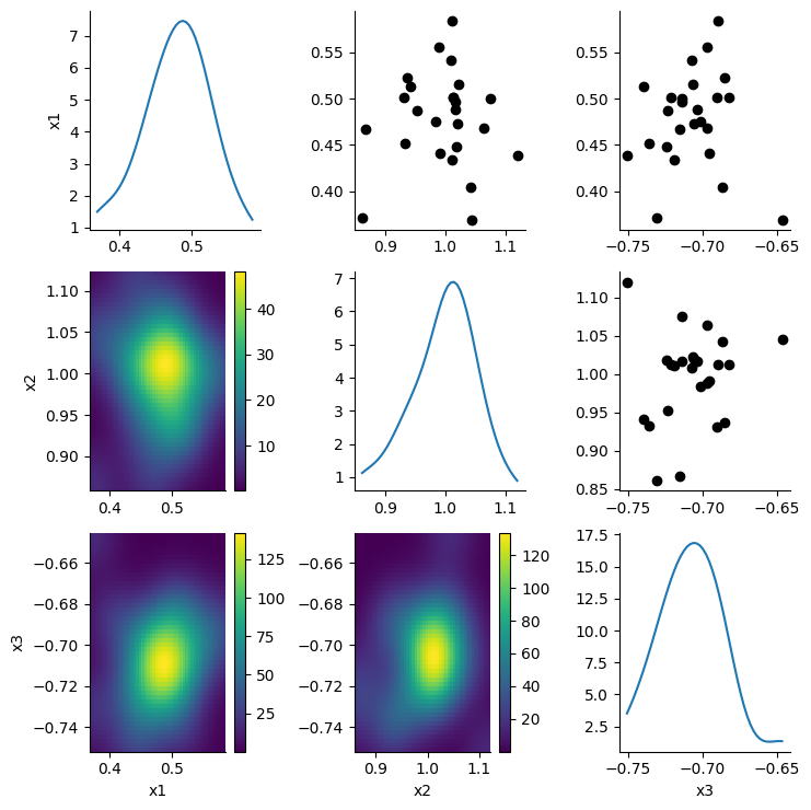
The calibrator is able to retrieve the ground-truth parameter values from our simulation study.

pd.DataFrame([
    { "parameter": estimate.name, "estimate": estimate.estimate, "ground truth": ground_truth[estimate.name] }
    for estimate in calibrator.get_parameter_estimates().estimates
])

	parameter	estimate	ground truth
0	x1	0.478148	0.5
1	x2	0.995373	1.0
2	x3	-0.707393	-0.7

Overall, TorchX is not required for computationally light-weight functions such as our R-based, Rastrigin function. However, it is more useful for computationally demanding simulations that must be executed in a distributed and parallelised fashion within a computing cluster.

For the examples above, we have set the TorchX scheduler to local_cwd. Hence, we are running the simulations locally. However, TorchX supports many different schedulers, and it’s worth experimenting with them.

pd.DataFrame(torchx.schedulers.get_scheduler_factories().keys())

	0
0	local_docker
1	local_cwd
2	slurm
3	kubernetes
4	kubernetes_mcad
5	aws_batch
6	aws_sagemaker
7	lsf