Custom Calibrators

The following tutorial demonstrates how one may create a custom calibrator to perform your own calibration workflows.

from matplotlib import pyplot as plt
import numpy as np
import pandas as pd
from scipy.optimize import differential_evolution

from calisim.base import CalibrationWorkflowBase
from calisim.data_model import (
	DistributionModel,
	ParameterDataType,
	ParameterSpecification,
)
from calisim.data_model import ParameterDataType, ParameterEstimateModel

from calisim.example_models import LotkaVolterraModel
from calisim.optimisation import OptimisationMethod, OptimisationMethodModel
from calisim.statistics import MeanSquaredError

import warnings
warnings.filterwarnings("ignore")

Creating a Calibrator

Let’s create a custom calibrator called SciPyDEOptimisation that uses SciPy’s differential evolution algorithm for calibrating models via black-box optimisation. All custom calibrators must inherit from the CalibrationWorkflowBase abstract class.

class SciPyDEOptimisation(CalibrationWorkflowBase):
    """The SciPy differential evolution optimisation method class."""

The CalibrationWorkflowBase class defines three abstract methods which must be implemented by your calibrator:

• specify(): Specify the parameters of the model calibration procedure.

• execute(): Execute the simulation calibration procedure.

• analyze(): Analyze the results of the simulation calibration procedure.

Specify

Let’s first define specify():

def specify(self) -> None:
    """Specify the parameters of the model calibration procedure."""
    self.names = []
    self.data_types = []
    self.bounds = []
    
    parameter_spec = self.specification.parameter_spec.parameters
    for spec in parameter_spec:
        parameter_name = spec.name
        data_type = spec.data_type
    
        if data_type == ParameterDataType.CONSTANT:
            parameter_value = spec.parameter_value
            self.constants[parameter_name] = parameter_value
            continue
        elif data_type == ParameterDataType.CATEGORICAL:
            bounds = self.set_categorical_parameter(spec)
        else:
            bounds = self.get_parameter_bounds(spec)  
    
        self.names.append(parameter_name)
        self.data_types.append(data_type)
        self.bounds.append(bounds)

We can see that our calibrator loops through each parameter specification within a ParameterSpecification collection object.

CalibrationWorkflowBase has a constants dictionary for storing CONSTANT parameter data types. CalibrationWorkflowBase defines a method called set_categorical_parameter() for dealing with CATEGORICAL data, which returns lower and upper parameter bounds. For CONTINUOUS and DISCRETE data, CalibrationWorkflowBase defines a method called get_parameter_bounds() which returns the lower and upper parameter bounds.

Finally, we store the parameter names, data types, and bounds within three lists.

Execute

Let’s next define execute():

def execute(self) -> None:
    """Execute the simulation calibration procedure."""
    optimisation_kwargs = self.get_calibration_func_kwargs()

    self.history = []
    self.eval_count = 0
    output_labels = self.specification.output_labels
    if output_labels is None:
        output_labels = ["target"]
        
    def target_function(X: np.ndarray) -> np.ndarray:
        X_dict = {
            name: X[i]
            for i, name in enumerate(self.names)
        }
        X = [X]
        
        Y = self.calibration_func_wrapper(
            X,
            self,
            self.specification.observed_data,
            self.names,
            self.data_types,
            optimisation_kwargs,
        )

        X_dict["eval_count"] = self.eval_count
        self.eval_count += 1
        X_dict[output_labels[0]] = Y
        self.history.append(X_dict)
    
        return Y
    
    n_iterations = self.specification.n_iterations
    verbose = self.specification.verbose
    n_jobs = self.specification.n_jobs
    random_seed = self.specification.random_seed

    method_kwargs = self.specification.method_kwargs
    if method_kwargs is None:
        method_kwargs = {}
            
    self.study = differential_evolution(
        target_function,
        self.bounds,
        maxiter=n_iterations,
        disp=verbose,
        workers=n_jobs,
        seed=random_seed,
        **method_kwargs
    )

The CalibrationWorkflowBase class defines a getter method called get_calibration_func_kwargs() that retrieves the calibration_func_kwargs values supplied to the OptimisationMethodModel object’s constructor. This allows us to include custom arguments within our objective function.

Our SciPyDEOptimisation class will store the trial history and number of objective function evaluations using two properties (self.history and self.eval_count). We specify the names of our objectives using the output_labels field within our OptimisationMethodModel specification.

We define a function called target_function() which will be executed by the differential evolution algorithm. This function calls the calibration_func_wrapper() method, which is defined by our CalibrationWorkflowBase base class. calibration_func_wrapper() will perform some data preprocessing and call our objective function under the hood.

We retrieve several OptimisationMethodModel specification values:

• n_iterations: The number of trial iterations for optimisation.

• verbose: The verbosity of the calibration procedure. How much detail is provided in the outputs.

• n_jobs: The number of jobs to run for parallel processing.

• random_seed: The random seed for replicability due to stochasticity.

• method_kwargs: Named arguments to pass to the calibration procedure when the default values are insufficient.

Finally, we execute the differential_evolution() algorithm to perform calibration.

Analyze

We must next define analyze():

def analyze(self) -> None:
    """Analyze the results of the simulation calibration procedure."""
    task, time_now, experiment_name, outdir = self.prepare_analyze()

    output_labels = self.specification.output_labels
    if output_labels is None:
        output_labels = ["target"]
        
    trials_df = pd.DataFrame(self.history)
    trials_df_best = trials_df.sort_values(output_labels).head(1)
    for col in trials_df_best.columns:
        if col in output_labels or col == "eval_count":
            continue
        estimate = trials_df_best[col].item()
        parameter_estimate = ParameterEstimateModel(name=col, estimate=estimate)
        self.add_parameter_estimate(parameter_estimate)

    for output_label in output_labels:
        ax  = trials_df.plot.scatter("eval_count", output_label, figsize=self.specification.figsize)
        fig = ax.get_figure()
        ax.set_title(f"Optimisation history: {output_label}")
        
        self.present_fig(
            fig, outdir, time_now, task, experiment_name, f"plot-optimization-history-{output_label}"
        )

    fig, axes = plt.subplots(nrows = len(self.names), figsize=self.specification.figsize)
    for i, name in enumerate(self.names):
        trials_df.plot.scatter(name, "eval_count", ax=axes[i])
        axes[i].invert_yaxis()
        axes[i].set_title(f"Parameter: {name}")
    self.present_fig(
        fig, outdir, time_now, task, experiment_name, "plot-slice"
    )
        
    if outdir is None:
        return
    
    self.to_csv(trials_df, "trials")

The prepare_analyze() method retrieves several values which are needed to store data to file.

From our self.history property, we can construct a trial history Pandas dataframe. We retrieve the best trial from the dataframe, and thereafter save the optimised parameter estimates within ParameterEstimateModel objects, which are then added to a list of parameter estimates via the add_parameter_estimate() method.

We loop through each named objective (output_labels) and construct a scatter plot visualising the relationship between the objective values and the trial evaluation number. The CalibrationWorkflowBase class defines the present_fig() method which will either save the scatter plot to file or directly render and open the plot to the user’s screen. We also loop through each named parameter (self.names) and similarly create scatter plots to visualise the relationship between parameter values and the trial evaluation number.

Finally, if the outdir directory is provided, we save the trial history dataframe as a csv file.

Let’s put all of this code together into one SciPyDEOptimisation class:

class SciPyDEOptimisation(CalibrationWorkflowBase):
    """The SciPy differential evolution optimisation method class."""

    def specify(self) -> None:
        """Specify the parameters of the model calibration procedure."""
        self.names = []
        self.data_types = []
        self.bounds = []
        
        parameter_spec = self.specification.parameter_spec.parameters
        for spec in parameter_spec:
            parameter_name = spec.name
            data_type = spec.data_type
        
            if data_type == ParameterDataType.CONSTANT:
                parameter_value = spec.parameter_value
                self.constants[parameter_name] = parameter_value
                continue
            elif data_type == ParameterDataType.CATEGORICAL:
                bounds = self.set_categorical_parameter(spec)
            else:
                bounds = self.get_parameter_bounds(spec)  
        
            self.names.append(parameter_name)
            self.data_types.append(data_type)
            self.bounds.append(bounds)

    def execute(self) -> None:
        """Execute the simulation calibration procedure."""
        optimisation_kwargs = self.get_calibration_func_kwargs()

        self.history = []
        self.eval_count = 0
        output_labels = self.specification.output_labels
        if output_labels is None:
            output_labels = ["target"]
            
        def target_function(X: np.ndarray) -> np.ndarray:
            X_dict = {
                name: X[i]
                for i, name in enumerate(self.names)
            }
            X = [X]
            
            Y = self.calibration_func_wrapper(
                X,
                self,
                self.specification.observed_data,
                self.names,
                self.data_types,
                optimisation_kwargs,
            )

            X_dict["eval_count"] = self.eval_count
            self.eval_count += 1
            X_dict[output_labels[0]] = Y
            self.history.append(X_dict)
        
            return Y
        
        n_iterations = self.specification.n_iterations
        verbose = self.specification.verbose
        n_jobs = self.specification.n_jobs
        random_seed = self.specification.random_seed

        method_kwargs = self.specification.method_kwargs
        if method_kwargs is None:
            method_kwargs = {}
                
        self.study = differential_evolution(
            target_function,
            self.bounds,
            maxiter=n_iterations,
            disp=verbose,
            workers=n_jobs,
            seed=random_seed,
            **method_kwargs
        )

    def analyze(self) -> None:
        """Analyze the results of the simulation calibration procedure."""
        task, time_now, experiment_name, outdir = self.prepare_analyze()

        output_labels = self.specification.output_labels
        if output_labels is None:
            output_labels = ["target"]
            
        trials_df = pd.DataFrame(self.history)
        trials_df_best = trials_df.sort_values(output_labels).head(1)
        for col in trials_df_best.columns:
            if col in output_labels or col == "eval_count":
                continue
            estimate = trials_df_best[col].item()
            parameter_estimate = ParameterEstimateModel(name=col, estimate=estimate)
            self.add_parameter_estimate(parameter_estimate)

        for output_label in output_labels:
            ax  = trials_df.plot.scatter("eval_count", output_label, figsize=self.specification.figsize)
            fig = ax.get_figure()
            ax.set_title(f"Optimisation history: {output_label}")
            
            self.present_fig(
                fig, outdir, time_now, task, experiment_name, f"plot-optimization-history-{output_label}"
            )

        fig, axes = plt.subplots(nrows = len(self.names), figsize=self.specification.figsize)
        for i, name in enumerate(self.names):
            trials_df.plot.scatter(name, "eval_count", ax=axes[i])
            axes[i].invert_yaxis()
            axes[i].set_title(f"Parameter: {name}")
        self.present_fig(
            fig, outdir, time_now, task, experiment_name, "plot-slice"
        )
            
        if outdir is None:
            return
        
        self.to_csv(trials_df, "trials")

Performing Calibration

That covers the end-to-end process of creating a custom calibrator. Let’s try calibrating an example model: LotkaVolterraModel.

model = LotkaVolterraModel()
observed_data = model.get_observed_data()
observed_data.head(5)

	year	lynx	hare
0	1900.0	4.0	30.0
1	1901.0	6.1	47.2
2	1902.0	9.8	70.2
3	1903.0	35.2	77.4
4	1904.0	59.4	36.3

We’ll define our parameter specification containing parameter names, data types, distribution types, and bounds.

parameter_spec = ParameterSpecification(
	parameters=[
		DistributionModel(
			name="alpha",
			distribution_name="uniform",
			distribution_args=[0.45, 0.55],
			data_type=ParameterDataType.CONTINUOUS,
		),
		DistributionModel(
			name="beta",
			distribution_name="uniform",
			distribution_args=[0.02, 0.03],
			data_type=ParameterDataType.CONTINUOUS,
		),
	]
)

We’ll define our objective function. We aim to minimise the discrepancy between simulated and observed data using the MeanSquaredError metric as our loss.

def objective(
	parameters: dict, simulation_id: str, observed_data: np.ndarray | None, t: pd.Series
) -> float | list[float]:
	simulation_parameters = dict(h0=34.0, l0=5.9, t=t, gamma=0.84, delta=0.026)

	for k in ["alpha", "beta"]:
		simulation_parameters[k] = parameters[k]

	simulated_data = model.simulate(simulation_parameters).lynx.values
	metric = MeanSquaredError()
	discrepancy = metric.calculate(observed_data, simulated_data)
	return discrepancy

We’ll define the specification for the differential evolution optimisation procedure. This will include the number of opimisation iterations (n_iterations), the name of the optimisation objectives (output_labels), and the named arguments to pass to SciPy’s differential evolution function (method_kwargs).

specification = OptimisationMethodModel(
	experiment_name="scipy_optimisation",
	parameter_spec=parameter_spec,
	observed_data=observed_data.lynx.values,
	n_iterations=100,
	output_labels=["Lynx"],
	method_kwargs=dict(
		init='latinhypercube',
        popsize=15
	),
	calibration_func_kwargs=dict(t=observed_data.year),
)

Finally, let’s run the calibration workflow by instantiating an OptimisationMethod calibrator, and subsequently calling the specify(), execute(), and analyze() methods.

calibrator = OptimisationMethod(
	calibration_func=objective, 
    specification=specification, 
    implementation=SciPyDEOptimisation
)

calibrator.specify().execute().analyze()

<calisim.optimisation.implementation.OptimisationMethod at 0x7fbde9e427a0>

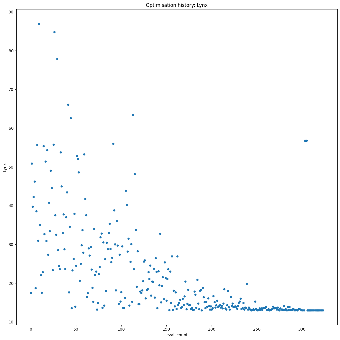
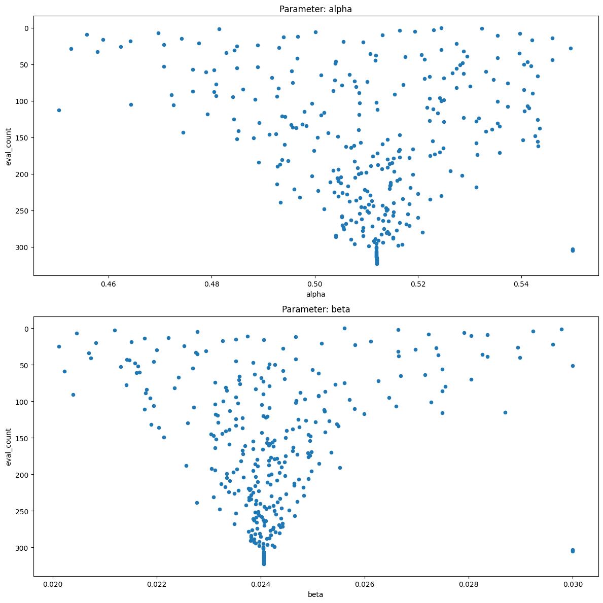
The differential evolution algorithm was able to recover the ground truth parameters for the simulation study.

pd.DataFrame([
    { "parameter": estimate.name, "estimate": estimate.estimate, "ground truth": model.GROUND_TRUTH[estimate.name] }
    for estimate in calibrator.get_parameter_estimates().estimates
])

	parameter	estimate	ground truth
0	alpha	0.512032	0.520
1	beta	0.024060	0.024