Approximate Bayesian Computation

The following tutorial demonstrates how one may calibrate a simulation model via Approximate Bayesian Computation (ABC) using calisim. We will first import our required dependencies.

from calisim.data_model import (
	DistributionModel,
	ParameterDataType,
	ParameterSpecification,
)
from calisim.example_models import SirOdesModel
from calisim.abc import (
	ApproximateBayesianComputationMethod,
	ApproximateBayesianComputationMethodModel,
)
from calisim.statistics import L2Norm
import numpy as np
import pandas as pd
from scipy.integrate import solve_ivp

import warnings
warnings.filterwarnings("ignore")

SIR Model Parameters and Initial Conditions

We next define our forward model. We will use an SIR (susceptible, infected, and recovered) compartmental model, combined with SciPy’s solver for ordinary differential equations. The SIR model is expressed as a system of ordinary differential equations where:

Parameter	Value	Description
β (beta)	0.4	Infection rate: probability of transmission per contact per time unit
γ (gamma)	0.1	Recovery rate: fraction of infected recovering per time unit
		Average infectious period = 1 / γ = 10 time units

With the following compartments:

Compartment	Symbol	Initial Value	Description
Susceptible	S0	999	Individuals who can catch the disease (N - I0 - R0)
Infected	I0	1.0	Individuals currently infected and can spread the disease
Recovered	R0	0	Individuals recovered or removed; no longer infectious

def sir_simulate(parameters: dict) -> np.ndarray | pd.DataFrame:
    def dX_dt(_: np.ndarray, X: np.ndarray) -> np.ndarray:
        S, I, _ = X 
        dotS = -parameters["beta"] * S * I / parameters["N"]
        dotI = (
            parameters["beta"] * S * I / parameters["N"] - parameters["gamma"] * I
        )
        dotR = parameters["gamma"] * I
        return np.array([dotS, dotI, dotR])

    X0 = [parameters["S0"], parameters["I0"], parameters["R0"]]
    t = (parameters["t"].min(), parameters["t"].max())
    x_y = solve_ivp(
        fun=dX_dt, y0=X0, t_span=t, t_eval=parameters["t"].values.flatten()
    ).y

    df = pd.DataFrame(dict(dotS=x_y[0, :], dotI=x_y[1, :], dotR=x_y[2, :]))
    return df

We will perform a simulation study with the following ground-truth parameters:

model = SirOdesModel()
pd.DataFrame(model.GROUND_TRUTH, index=[0]) 

	beta	gamma	N	I0	R0	S0
0	0.4	0.1	1000	1.0	0	999.0

When supplied to our forward model, these ground-truth parameters will generate the observed data below:

observed_data = model.get_observed_data()
observed_data.head(6)

	dotS	dotI	dotR	day
0	999.000000	1.000000	0.000000	0
1	998.534208	1.349201	0.116592	1
2	997.906105	1.819995	0.273899	2
3	997.059813	2.454180	0.486007	3
4	995.919926	3.308098	0.771976	4
5	994.385263	4.457212	1.157524	5

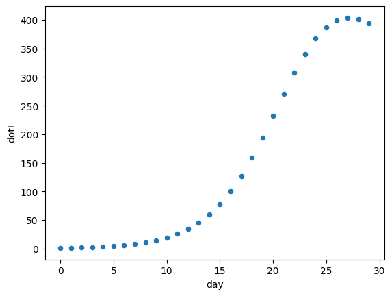
Let’s view the trajectory of infected individuals over time in days.

observed_data.plot.scatter("day", "dotI")

<Axes: xlabel='day', ylabel='dotI'>

Bayesian Calibration via Approximate Bayesian Computation Sequential Monte Carlo

Next, let’s use calisim to perform Bayesian calibration via ABC using the simulated and observed number of infections. We will apply the L2 norm as our distance metric, with the aim of minimising the discrepancy between simulated and observed data.

To start with, we’ll need to define our ParameterSpecification parameter specification using Normally distributed priors:

parameter_spec = ParameterSpecification(
	parameters=[
		DistributionModel(
			name="beta",
			distribution_name="normal",
			distribution_args=[0.35, 0.05],
			data_type=ParameterDataType.CONTINUOUS,
		),
		DistributionModel(
			name="gamma",
			distribution_name="normal",
			distribution_args=[0.08, 0.01],
			data_type=ParameterDataType.CONTINUOUS,
		),
	]
)

This contains information concerning the various parameter names, probability distributions, ranges, distribution parameters, and data types.

We next need to define a wrapper function around our forward model to ensure there’s compatibility with the calisim API.

def abc_func(
	parameters: dict, simulation_id: str, observed_data: np.ndarray | None, t: pd.Series
) -> float | list[float]:
    simulation_parameters = model.GROUND_TRUTH.copy()
    simulation_parameters["t"] = t
    
    for k in ["beta", "gamma"]:
        simulation_parameters[k] = parameters[k]
    
    simulated_data = sir_simulate(simulation_parameters).dotI.describe().values
    metric = L2Norm()
    discrepancy = metric.calculate(observed_data, simulated_data)
    return discrepancy

The last step is to create a ApproximateBayesianComputationMethodModel specification for the calibration procedure itself, which we then supply to a ApproximateBayesianComputationMethod calibrator. We’ll use the ABC Sequential Monte Carlo method via the pyABC engine.

specification = ApproximateBayesianComputationMethodModel(
	experiment_name="pymc_approximate_bayesian_computation",
	parameter_spec=parameter_spec,
	observed_data=observed_data.dotI.describe().values,
	n_init=25,
	walltime=1, 
	epsilon=0.1,
	n_bootstrap=15,
	min_population_size=5,
	output_labels=["Number of Infected"],
	calibration_func_kwargs=dict(t=observed_data.day),
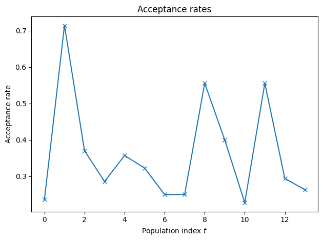
	method_kwargs=dict(max_total_nr_simulations=500, max_nr_populations=20, min_acceptance_rate=0.),
)

calibrator = ApproximateBayesianComputationMethod(
	calibration_func=abc_func, specification=specification, engine="pyabc"
)

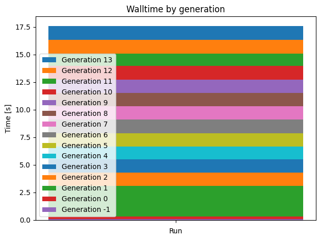
Finally, we’ll run the calibration procedure. This is composed of 3 steps:

1. Specify: Define your calibration problem: Parameter distributions, observed data, objective/discrepancy function, and calibration settings (like algorithm, directions, iterations)

2. Execute: Run the actual calibration process (simulation + optimization/inference)

3. Analyze: Process, summarize, and optionally save plots/metrics of the calibration results

Or SEA.

import logging
logging.getLogger("pyabc").setLevel(logging.INFO)
calibrator.specify().execute().analyze()

<calisim.abc.implementation.ApproximateBayesianComputationMethod at 0x7f7877fec6d0>

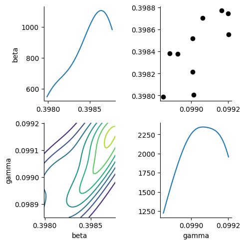
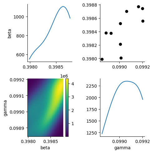
Let’s view the parameter estimates produced by the calibrator, with some measure of uncertainty.

pd.DataFrame([
    { "parameter": estimate.name, "estimate": estimate.estimate, "uncertainty": estimate.uncertainty, "ground truth": model.GROUND_TRUTH[estimate.name] }
    for estimate in calibrator.get_parameter_estimates().estimates
])

	parameter	estimate	uncertainty	ground truth
0	beta	0.398426	0.000286	0.4
1	gamma	0.099032	0.000126	0.1

The ABC calibrator is able to retrieve the ground-truth parameter values from our simulation study.